Basemath—GetYourGuide’s Way of Sequential Testing. Part II: The Theory

In part two of this two-part series, Senior Data Science Manager Alexander Weiss deep dives into the mechanics of Basemath, our open-source approach to A/B testing. Explore the mathematical foundation that ensures accuracy while adhering to error constraints, learn about our transition from continuous to discrete experiment evaluation, and more.

{{divider}}

In the introductory article on Basemath, GetYourGuide's open-source solution for sequential testing, you learned the application of the method. This follow-up article delves into the mechanics behind the scenes. Basemath approaches A/B testing as a random walk. We will begin by elucidating the link between A/B tests and random walks. Subsequently, we will discuss deriving a function that adheres to both type I and type II error constraints. The article will conclude with an explanation of transitioning from continuous to discrete evaluation of the experiment. Additionally, as an extra feature, we will provide a concise overview of what a spending function is and the specific spending function employed by Basemath.

A/B Experiments: A Random Walks Approach

Basemath evaluates two variants—the control and the treatment—each with an identical sample size. Every sample is assigned a value, which can be any real number. However, for the sake of simplicity, we will focus on the binary scenario where the value is designated as either 0 (failure) or 1 (success).

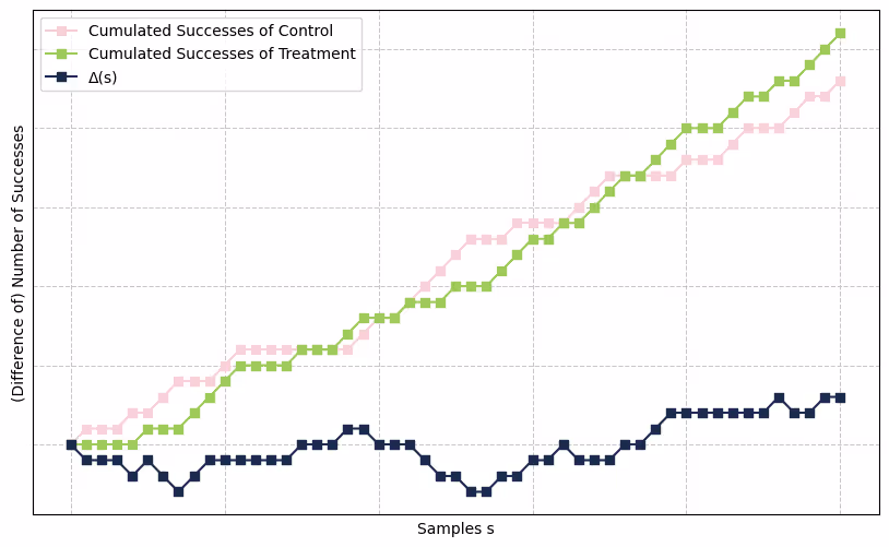
The figure above illustrates the cumulative number of successes for both the control group (in green) and the treatment group (in pink), plotted as a function of the increasing sample size for a specific experiment. The dark blue curve represents the difference between the successes of the treatment and the control groups. The function representing the difference after s samples is denoted by Δ(s). Operating under the premise that each sample may yield a value of 1 with a given probability of success and 0 with the complementary probability of failure, Δ exhibits certain probabilities of either rising by one step, descending by one step, or remaining constant at each point in the sequence. These probabilities are consistent at every step and are independent of the current value of the difference curve. Such behavior characterizes Δ as a specific type of random walk.

The subsequent figure presents the difference curves Δ_i derived from 2,000 simulated experiments. Half of these simulations, amounting to 1,000, were conducted with the control and treatment groups having identical probabilities of success, depicted in blue. The remaining 1,000 simulations were based on the premise that the treatment group enjoys a higher likelihood of success compared to the control, illustrated in red.

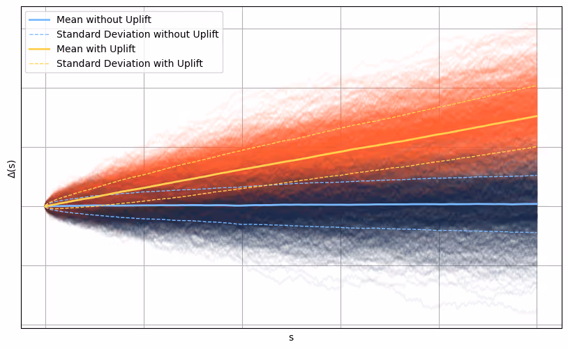
When both variants share an equal probability of success, the average difference between them typically hovers around zero, as represented by the solid light blue line in the figure. Naturally, random fluctuations are part of the process, and their expected magnitude is indicated by the dashed lines surrounding the average.

In scenarios where the treatment’s success probability surpasses that of the control, the difference curve exhibits a positive linear trend, highlighted by the solid yellow line. The scale of fluctuations remains comparable to those observed when success probabilities are equal.

As the sample size increases, a fascinating divergence occurs: the red curves, representing the experiments with a higher success probability for the treatment, begin to drift markedly away from the blue ones. This separation accelerates, with the gap between their respective averages widening at a rate that outpaces the growth of their fluctuations. This very characteristic empowers us to identify an uplift, provided the experiment is allowed to run for a sufficient duration.

With these insights, we are now primed to delve into the intricate workings of Basemath’s proof.

Basemath’s Proof

As a refresher, Basemath ensures that Prob(Type I error) ≤ α, and Prob(Type II error I MDE ≥ e)  ≤ β(e). Both α and β(e) are values ranging from 0 to 1 and serve as input parameters alongside e, which represents a bound on the minimal detectable effect (MDE) in percentage points. For a detailed explanation, please refer to the "What Basemath Tests" section in the preceding article.

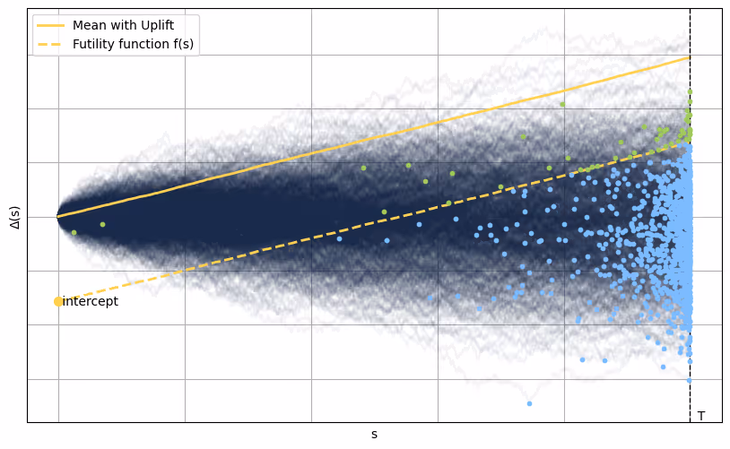
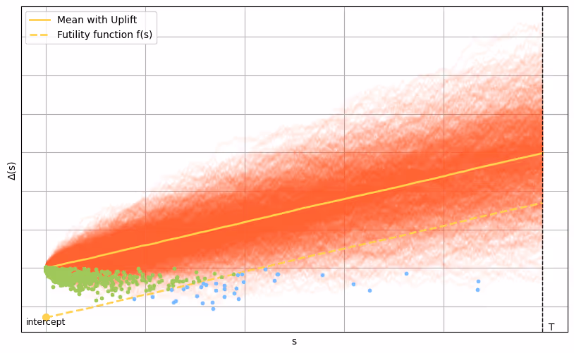
The two charts above illustrate the two scenarios separately: one demonstrating an uplift and the other lacking it. In both charts, the average trajectory of the uplift scenario, represented by a solid yellow line,  has a gradient of e. Furthermore, a circular marker accentuates the lowest point on each individual trajectory. The color of these markers varies, depending on whether they fall above or below the futility threshold, which is depicted as a dashed yellow line. This futility function, denoted as f(s), is defined by the equation f(s) = intercept + s * e.

A key observation is that determining whether a trajectory intersects with the futility function is essentially the same as ascertaining whether its lowest point is situated above or below this function. Consequently, the first criterion we aim to meet, which is that the probability of a type I error should be less or equal to α, can be interpreted as requiring that no more than an α proportion of all trajectories should have their minimum point above the futility function f within the interval [0, T], where T represents the maximum number of samples per variation. Similarly, for trajectories exhibiting an increase, we desire that no more than a β(e) proportion should have their minimum point below f within the same interval.

In conclusion, given a specified MDE e, we must identify the appropriate values for the intercept and T parameters to ensure that both type I and type II error constraints are simultaneously met.

In our study, we demonstrate that the specific intercept is dependent on the variable T in the following way:

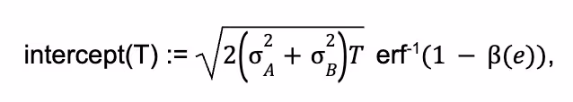
where σ² represents the variance of both the control group (A) and the treatment group (B). The term erf^-1 refers to the inverse error function.

Additionally, the intercept and the variable T are constrained by a particular condition that must be satisfied:

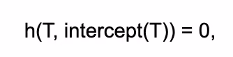
where the function h is given by:

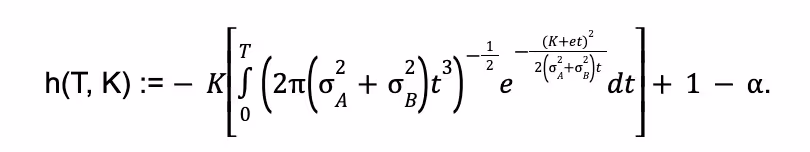
We establish that for each set of valid inputs  (α, β(e), e, σ_A, σ_B), there is a unique solution. This solution can be determined using a numerical root-finding technique.

From Continuous to Batch Evaluation

Thus far, we have operated under the assumption of continuous monitoring for our experiment. In reality, the function Δ is observed at discrete intervals, corresponding to our daily data evaluation process.

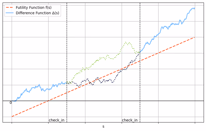
The graph displayed above illustrates a realization of Δ. It is assumed that the trajectory between two check-in points is unobservable. The green and the dark blue dotted lines represent two possible behaviors within this time frame. Both scenarios are equally probable and are merely two among thousands of potential realizations. The difficulty arises from the fact that, in the blue scenario, Δ intersects with the futility function, necessitating the termination of the experiment, whereas in the green scenario, it remains above. Since Δ is above the futility function at the subsequent check-in, one cannot determine the exact path taken in the interim with certainty.

We address this challenge by employing a probabilistic approach to determine whether to halt the experiment. Specifically, we decide to stop the experiment by flipping a coin, with the probability of stopping being contingent upon the likelihood of intersecting the futility function. This likelihood is calculated based on the distance of Δ from the futility threshold at the last and current check-ins, as well as the sample size between these two points. The probability of crossing is given by the formula:

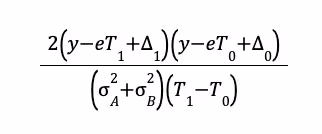
In this formula, y represents the intercept, T₀ and T₁ denote the check-in points, and Δ₀ and Δ₁ are the corresponding values of Δ at these points.

While it may seem unconventional to use a coin flip to decide an experiment’s outcome, this method is quite sophisticated from a statistical perspective. It obviates the need to adjust the futility function at each check-in, a practice characteristic of traditional methods that typically requires numerical integration at every check-in point.

Bonus: The Spending Function

You may be curious about the likelihood of your experiment being prematurely terminated due to reaching the futility threshold. The answer to this question is provided by the spending function. Specifically, the boundary for a type II error is denoted by β(e), meaning that a proportion β(e) of all realizations of Δ that actually exhibit an uplift will be prematurely halted and incorrectly classified as flat before reaching the maximum sample size. Nonetheless, the experiment will cease earlier if these realizations encounter the futility function.

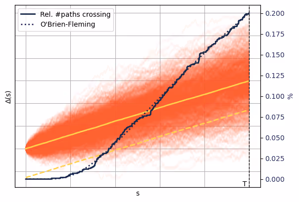
The graph above illustrates the proportion of sampled trajectories that have encountered the futility function up to a given sample size “s,” represented by the dark blue line. Note that it reaches the level of β(e) = 20% at the maximum sample size “T”. Beneath the solid blue line is another dotted line representing the O’Brien-Fleming spending curve, a widely recognized spending function. The function is defined as follows:

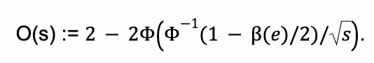
This curve is characterized by its conservative approach at experiment’s outset, transitioning to a more linear behavior in the later stages. Such a design ensures we do not terminate an experiment with insufficient evidence.

‍