Basemath—GetYourGuide’s Way of Sequential Testing. Part I: The Application

Discover Basemath—GetYourGuide's open-source solution for sequential testing. In part one of this two-part series, Senior Data Science Manager Alexander Weiss shares the methodology behind Basemath, input requirements, and how to put it into action.

{{divider}}

Sequential testing effectively reduces the run time of A/B tests, which are the gold standard for evaluating new features. Shortening A/B test running times at scale was particularly interesting to us because we knew it could significantly increase our velocity for shipping new features to customers, resulting in greater customer impact. Our article How Sequential Testing Accelerates Our Experimentation Velocity gives an excellent overview of our general journey to sequential testing.

There are many different approaches to sequential testing. At GetYourGuide, we developed our own easy-to-understand and easy-to-use method that provides lightning-fast evaluation of experiments. We call our approach Basemath, named after the daughter of King Solomon.

This article will explain exactly what you are testing for when using Basemath, the input it requires, and how to implement our open-source solution.

In a follow-up article, we will dive deeper into the statistical principles behind our approach and explain what makes it faster and simpler than other approaches.

What Basemath Tests

Basemath works on A/B tests with two variants: a control and a treatment. The traffic is equally distributed so that each variant receives 50% of the sample size. Each sample records a value. In binary tests, the value is either 0 (failure) or 1 (success). In continuous tests, the value can be any real number. For example, visitors to a platform could represent samples. In binary tests, samples could indicate whether a visitor converted into a customer ( 1 ) or churned before purchasing ( 0 ). For continuous tests, the value could be the revenue generated by each visitor, including 0 for non-customers. Basemath evaluates whether the average value per visitor is significantly higher for the treatment variant in both scenarios. This average value per sample is the experiment’s target metric, calculated as the sum of all sample values divided by the total number of samples per variant.

There are two types of errors we want to control for. A Type I error assumes the test reports a significant uplift for the treatment versus the control when, in reality, the variants are equal on the target metric or the control performs even better than the treatment. A Type II error assumes we fail to detect an existing uplift. For Type II errors, we must specify a minimal detectable effect—MDE—the smallest uplift we want to be able to detect. Otherwise, the sample size required to reach a conclusion would be infinite.

Basemath guarantees Prob(Type I error) ≤ α, and Prob(Type II error I MDE ≥ e)  ≤ β(e). α and β(e) are values between 0 and 1 that are input parameters, along with e. α is also called the significance level; 1-β is called the statistical power. As we only test for an uplift of the treatment, Basemath conducts a one-sided test. Based on these inputs, Basemath calculates the maximum required sample size.

Most companies don’t evaluate experiments in real-time, sample by sample. Typically, as with GetYourGuide, experiments are evaluated daily. Basemath is designed for this use case, expecting aggregated A/B test data in batches - a group sequential testing approach.

When evaluating a new batch, Basemath will reach one of three conclusions. If the total samples haven’t exceeded the maximum, the data may be too ambiguous for a final decision, and more is needed. Or it may decide on the null hypothesis: the treatment is no better than the control and cannot be rejected. Once reaching the maximum without experiencing the previous two events, Basemath will reject the null, concluding the treatment significantly outperforms the control.

In summary, Basemath stops early if the experiment doesn’t look promising but fully exploits the running time—represented by the maximal sample size—if the treatment outperforms the control. Some sequential testing approaches stop early if a significant uplift is visible, continuing only if there’s no uplift or  underperformance. Our approach is preferable for two reasons: most experiments fail in practice, so stopping earlier for this larger share results in greater overall time savings. Also, underpowered experiments with little data showing a “significant” uplift may produce an undesirable abundance of false positives, so validity concerns are reduced. Read A/B Testing Intuition Busters: Common Misunderstandings in Online Controlled Experiments for more details on these issues.

Basemath Applied

The Ingredients

First, install our open-source Python package basemath-analysis via your package manager to run the analysis.

Basemath requires the following key inputs for each experiment:

• Significance level [α] - The maximum acceptable probability of reporting a false positive. Usually set to 0.05 or lower.
• (1 - Statistical power) [β] - The likelihood of not detecting an effect of a given size. Usually set to 0.2 or lower.
• Minimum Detectable Effect [MDE] - The minimum scientifically or practically important difference between variants.
• Baseline metric value - The average value of the target metric before the experiment starts. You can also use the control variant’s initial batch to compute it.
• Baseline metric variance [only for the continuous case] - The variance is calculated as the squared difference between each value and the average, summed for all values, and divided by count.
• Experiment name - A unique string (e.g. “checkout-blue-button-v2”) to identify this experiment ensures consistent results on repeat analysis.

Specifying these key inputs allows Basemath to evaluate your experiment data accurately.

The Application

You can evaluate a binary experiment using Basemath by:

1. Importing the Basemath package:

import basemath_analysis.basemath as bm

2. Creating an instance of the BaseMathsTest class:

bm_test = bm.BaseMathsTest(
      avg_A,
      mde,
      alpha,
      beta,
      var_A=var_A,
      seed="experiment_name"
)

Where:

• avg_A is the baseline metric value
• mde is the (relative) minimum detectable effect size
• alpha is the significance level
• beta is the (1-power)
• var_A is the variance of the baseline metric (only for continuous case)
• seed is the experiment name

var_A must be left away in case of a binary target metric.

3. Calling evaluate_experiment() and passing in the batch data:

bm_test.evaluate_experiment(
       prev_delta_successes, 
      delta_successes,
      prev_num_samples,
      num_samples
)

Where:

• prev_delta_successes denotes the sum of values in the treatment variant minus the sum of values in the control variant from the start of the experiment until the previous evaluation check-in. This value will be 0 for the first batch.
• delta_successes denotes the difference between the sum of values for the treatment and control variants for the most recent batch, between the previous check-in and the current one.
• prev_num_samples denotes the total number of samples in one variant from the start of the experiment until the previous evaluation check-in. This value will be 0 for the first batch.
• num_samples denote the number of samples included in the most recent batch.

4. Interpreting the return value:

The method will return 0 if the experiment is inconclusive and requires more data, -1 if the null hypothesis can be accepted, or 1 if the maximum sample size is reached and the null hypothesis can be rejected. 

5. Continue repeating steps 3-4 as you receive new batch data, evaluating the experiment continuously until it returns -1 or 1. At this point, you must stop testing to avoid violating Basemath’s assumptions.

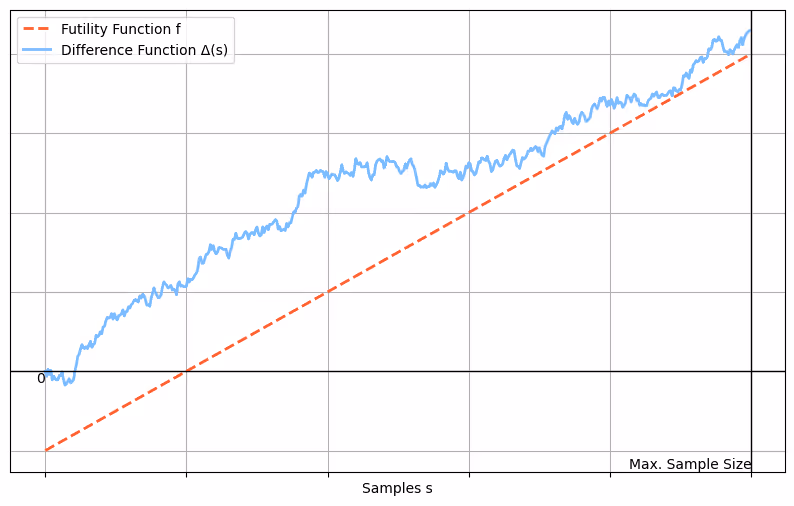
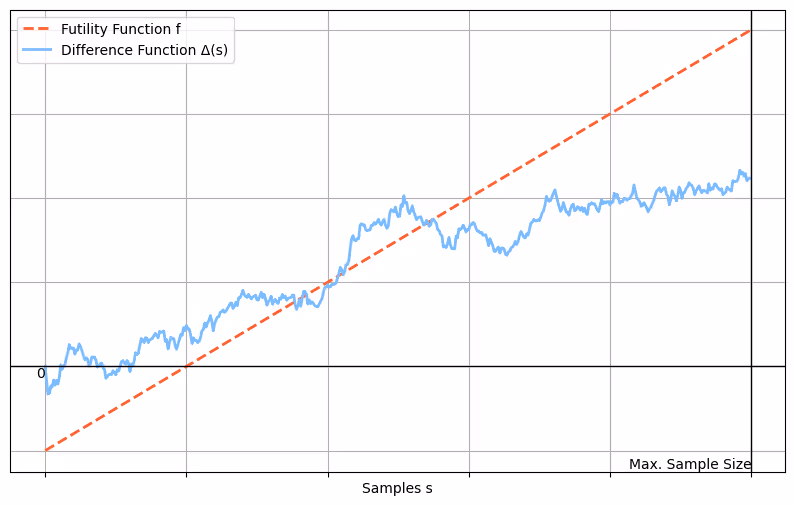
The Visualization

An instance of the BaseMathsTest class contains all the necessary information to visualize Basemath’s decision-making process. By calling,

(required_samples, intercept) = (
			bm_test.required_samples, bm_test_intercept
)

you can obtain the required sample size and intercept value from the BaseMathsTest object. You define the binding futility function f as:

f(s) = intercept + s * mde

where “s” denotes the number of samples seen so far in the experiment for one variant. Additionally, define the difference function Δ as:

Δ(s) = sum_of_successes_treatment - sum_of_successes_control

Δ(s) represents the difference between the sums of all sample values for the treatment and control groups at a given number of samples s.

As long as Δ(s) > f(s) and s is less than the required number of samples, Basemath will return 0. If Δ(s) ≤ f(s) for any s less than the required number of samples, it returns -1. If Δ(s) does not fall below f(s) before s reaches the required number of samples, Basemath returns 1.

These results are exact if Δ and f can be observed at all sample points s. However, if Δ and f can only be evaluated at particular check-in points s_1, s_2, etc., Basemath may return -1 even if Δ does not dip below f for any specific s_n.

Sounds strange? Yes! Want to learn why it’s nevertheless correct? Read the second part of this blog article about the mathematical foundations of Basemath!