GetYourGuide’s approach to A/B testing for ranking metrics: implementing clustered standard errors

When analyzing experiments in the data products team at GetYourGuide, we’ve faced numerous challenges evaluating the performance of our search. One particular statistical issue consistently arises when calculating significance in the online evaluations of ranking systems. Today, I’d like to share how we approach this problem using clustered standard errors and explain how this approach can benefit you as well.

{{divider}}

The problem: Unit of randomization <> Unit of analysis

Imagine you’re planning a trip to Rome. You might search for ’things to do in Rome’ multiple times over a week — maybe on your phone during lunch, on your laptop at home, or at other locations. Each search generates a ranking request. But here’s the catch: all those requests are assigned to the same experiment variant because assignment occurs at the visitor level.

When evaluating our ranking systems, we aim to measure metrics at the ranking request level. One of the standard metrics we track is booking Mean Average Precision (MAP) or NDCG (Normalized Discounted Cumulative Gain), calculated across all ranking requests (see this Wikipedia article for more common metrics in the space).

However, there’s a fundamental issue with this approach: a single visitor may generate multiple ranking requests! This creates a statistical challenge because the independence assumption of our A/B tests no longer applies. Going back to our Rome example, each search the traveler made influenced the subsequent ones. This means that ranking requests from the same visitor are inherently correlated and not independent trials.

2. Identifying where complexity lies: in the Metrics vs. in the Sampling Structure

My first instinct was to use the bootstrapping with our ranking request grain dataset. This turned out to be much more complex than that, which brought me to the point I want to unpack: not all complexity is created equally. Here are two main complexity sources that can help us better learn what we are dealing with:

1. The metric calculates percentiles or has any other complex structure (e.g., median revenue per visitor).
2. The unit of randomization (e.g., visitors) and unit of analysis (e.g., ranking requests) differ, introducing complexity in the sampling structure.

The former is solved by bootstrapping right away, while the latter requires a method that passes on the sampling hierarchy. A few options in this regard include sampling for bootstrapping at the visitor level, calculating the covariance for the delta method using visitor-level data, or adjusting the standard errors to account for it. 

The latter approach is somewhat less common in experimentation and is what we will talk about in this post. The reason we chose this approach instead of applying the delta method is twofold:

• Historical reasons: This corrected a previously incorrect implementation that had assumed each ranking request was independent.
• To preserve the test structure: Our pipeline calculates other t-tests, and we preferred a solution that fits into that mold.

What happens if we ignore the sampling problem completely?

If we analyze our data without accounting for this complex sampling structure, we risk overconfidence in our results. Our p-values may appear smaller than they should be, leading to narrower confidence intervals and potentially misleading us into declaring “significant” results that aren’t actually statistically significant. This increases our false positive rate — a dangerous outcome when making product decisions and determining the direction we need to take with our data product.

Introducing (clustered) standard errors

As presented above, one way to tackle this problem is to use a technique that’s well-established in economics but not very popular in tech: clustered standard errors.

Before diving into clustering, let’s clarify that standard errors represent the uncertainty in our estimated treatment effect. When we calculate a treatment effect, the standard error tells us how much that estimate might vary if the experiment were repeated. The standard error formula fundamentally depends on one critical assumption: independence of observations. The key underlying insight is that the standard error decreases with √n, because each additional independent observation reduces our uncertainty.

However, when observations within a cluster are correlated, your effective sample size is smaller than your total number of observations. If every ranking request from the same visitor were perfectly correlated (they either all convert or none convert), your effective sample size would just be the number of visitors, not the number of requests. In reality, correlation is partial, so the truth lies somewhere between the two extremes.

Clustered standard errors handle this by:

1. Recognizing the hierarchical structure (visitors → requests)
2. Estimating the within-cluster correlation
3. Adjusting the standard errors accordingly

Comparing the delta method and clustered standard errors

The problem we tackle in this blog post can be solved in multiple ways; the most popular is the delta method, and an alternative is clustered standard errors. I want to share the learnings on how similar those two are. Although there is already academic evidence of equivalence between the delta method and clustered standard error in the canonical form (see the paper), I did not find a converse explanation of the fundamental differences, which is what I aim to highlight here.

When we have random variables as numerator and denominator, the delta method computes the aggregated metrics first, and then addresses the unit of randomization vs the unit of analysis by estimating the variance of the ratio using the Taylor series. In the case of our visitors, the clusters reflect the data hierarchy — see this paper and Statsig’s/Eppo’s implementation for more details on clusters in the delta method.

The approach of clustered standard error is completely different. It preserves the shape of the metrics at the individual level (each data pair that contributes to the ratio metric is retained as such) and only accounts for the data hierarchy when calculating the standard error. It then performs the correction towards the end.

The delta method calculates the aggregates, and only then do the corrected values make sense. Clustered standard errors keep the metrics in the same form and shape as if you would calculate them by hand, without considering the unit of randomisation<>analysis differences. 

Both methods lead to the same destination. If you want to prioritize consistency with other t-tests, for example, then clustered standard errors will make the analysis easier to read through and implement. If you care only about the aggregates, then the delta method may be easier to implement in your data warehouse.

3. T-test: Moving from Standard Standard Errors to Clustered Ones

While most data practitioners are familiar with the t-test, not all of us are aware that a t-test is actually a special case of linear regression. This connection is crucial because it enables us to leverage robust variance estimation techniques, such as clustered standard errors, and incorporate them into the t-test.

The Connection Between t-tests and Linear Regression

In a simple A/B test, we can represent our model as:

Y = β₀ + β₁X + ε

Where:

• Y is our metric of interest
• X is a dummy variable (0 for control, 1 for treatment)
• β₀ is the mean of the control group
• β₁ is the difference between treatment and control (our effect)
• ε is the error term

The t-statistic for β₁ in this regression is exactly the same as the t-statistic from a two-sample t-test comparing the means.

Implementing Clustered Standard Errors

To account for clustering at the visitor level, we need to adjust our standard error calculations. The rest remains untouched. In Python, we can implement this using the statsmodels package:

import statsmodels.api as sm
from statsmodels.formula.api import ols

# Run regression with clustered standard errors
model = ols('value ~ group_dummy', data=df).fit(
    cov_type='cluster', 
    cov_kwds={'groups': df['visitor_id']}
)

# View results
print(model.summary().tables[1])

The mathematical intuition behind Clustered Standard Errors

Note: If you’re comfortable with statistics, this section will help you understand what’s happening “under the hood” of clustered standard errors. If you’re more interested in practical application, feel free to skip to the next section.

As far as train_predict() goes, it’s important to understand what is happening behind the scenes. The key insight: when observations within a cluster are correlated, your effective sample size is smaller than your total number of observations. This happens because a correlated or non-correlated observation adds different levels of information.

Taking it to an extreme, if every ranking request from the same visitor were perfectly correlated, you’d effectively have just the number of visitors as your sample size, not the number of requests. 

In reality, correlation is partial, so the truth lies somewhere in between. This is why the standard error formula is adapted.

Here’s what it looks like in a toy example: 

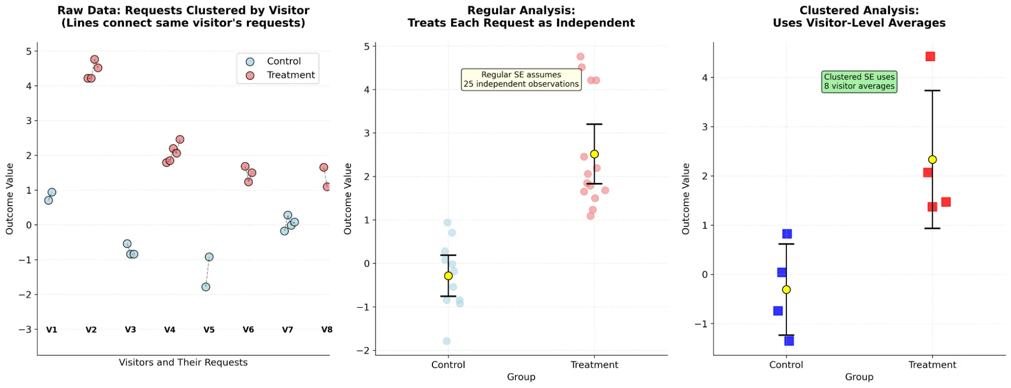
The three panels show exactly what’s happening:

1. Left panel: Shows the raw data where dots connected by lines represent the same visitor (V1-V8). Notice how requests from the same visitor tend to be similar (correlated).
2. Middle panel: Shows what regular analysis does - treats each dot as independent, giving narrow confidence intervals.
3. Right panel: Shows what clustered analysis does - first averages within each visitor (squares), then analyzes those averages, giving wider (more honest) confidence intervals.

In a nutshell, this method:

1. Recognizes the clustering structure: Instead of treating all requests as independent pieces of information, it recognizes that we actually have 8 visitors providing information.
2. Accounts for within-cluster correlation: The method doesn’t just average within clusters — it uses the “sandwich estimator” that adjusts the variance-covariance matrix to account for correlation.
3. Inflates uncertainty appropriately: Standard errors become larger, making t-statistics smaller and p-values more conservative.

4. Our application in ranking and potential problem spaces

When applying this method to our ranking data, we observed the most change in price-related metrics. Clustered standard errors increase the standard error of the regression coefficient β and widen the confidence intervals by around 30% increasing the p-value as a result (making it harder to have p-value fall under 0.05). This is vital because it allows us to understand the effect of our experiments on prices in a trustworthy manner, rather than having overconfidence in incorrect results.

In terms of the potential problem spaces, this approach could also be valuable for:

1. Analyzing performance metrics like Largest Contentful Paint (LCP) using percentiles
2. Checking the effects of imagery in an activity card by computing p-values and confidence intervals on clicks per impression
3. Evaluating autocompleter performance
4. All cases in which we analyze multiple observations of a given user.

An underlying, core principle to keep in mind? Whenever your data has a hierarchical structure, account for that structure in your statistical analysis to ensure accurate analysis and draw informed conclusions. 

5. Implementation at scale on PySpark

At GetYourGuide, we process millions of recommendations daily, so computational efficiency is crucial for this sort of analysis. While packages like statsmodels work well for small datasets, we needed to reimplement the core algorithms for our distributed computing environment using PySpark.

Inspired by the implementation in statsmodels, we had to adapt for our scale. Large language models proved surprisingly helpful in developing and debugging this implementation.

Recommended reading

For those interested in diving deeper into clustered standard errors and their applications, I highly recommend these resources:

1. Clustered Standard Errors in A/B Tests - A practical guide to implementing clustered standard errors specifically for A/B testing scenarios.
2. https://economics.mit.edu/sites/default/files/2022-09/When%20Should%20You%20Adjust%20Standard%20Errors%20for%20Clustering.pdf - theoretical background on when and how this makes sense.

Takeaways for experimenters

If you’re evaluating systems where the unit of assignment (like visitors) differs from the unit of analysis (like ranking requests), remember:

1. Check your assumptions: Independence is a critical assumption in statistical tests.
2. Know your sampling structure: Understand how users are assigned to variations.
3. Be cautious of overconfidence: Regular standard errors can lead to false positives.

These techniques can help us correctly assess significance in complex experimental settings, allowing us to think critically about our sampling structures and statistical approaches.

By properly accounting for the hierarchical structure in our data, we ensure that our significance tests are accurate, leading to informed decision-making and, ultimately, better experiences for every GetYourGuide user planning their next trip.

Want to pioneer your own path and shape the way millions of travelers experience the world? Check out our open roles here.

{{divider}}

Appendix: Full example — simulating and analyzing clustered data

To really understand how this works, let's look at a complete example. The following code simulates visitor data with clustering and demonstrates the impact of accounting for this structure:

 
import numpy as np
import pandas as pd
import scipy.stats as stats
import matplotlib.pyplot as plt
import uuid
from statsmodels.formula.api import ols
import statsmodels.api as sm

# Set random seed for reproducibility
np.random.seed(42)

# Define parameters
n_visitors = 100000  # Total number of visitors
control_mean = 0.492
treatment_mean = 0.492 * 1.02
std_dev = 8

# Generate visitor-level data
visitor_ids = [f"visitor_{i}" for i in range(n_visitors)]
# Assign visitors to groups (50/50 split)
visitor_groups = np.random.choice(['A', 'B'], size=n_visitors, p=[0.5, 0.5])
# Create visitor DataFrame
visitor_df = pd.DataFrame({
    'visitor_id': visitor_ids,
    'group': visitor_groups
})

# Generate visitor-specific treatment effects (some visitors respond more strongly than others)
# Base effect plus visitor-specific random component
visitor_df['base_value'] = np.random.normal(0, 5, n_visitors)  # Random baseline for each visitor
visitor_df['treatment_effect'] = np.where(
    visitor_df['group'] == 'B',
    np.random.normal(treatment_mean - control_mean, 5, n_visitors),  # Variable treatment effect
    0  # No effect for control group
)

# Determine number of rankings per visitor based on specified distribution
# 60% have 1 ranking, 20% have 2 rankings, 20% have 3 rankings
n_rankings = np.random.choice([1, 2, 10], size=n_visitors, p=[0.4, 0.2, 0.4])
visitor_df['n_rankings'] = n_rankings

# Generate ranking-level data
rankings_data = []
for i, row in visitor_df.iterrows():
    visitor_id = row['visitor_id']
    group = row['group']
    base_value = row['base_value']
    treatment_effect = row['treatment_effect']

    for j in range(row['n_rankings']):
        # Generate a unique ranking_uuid
        ranking_uuid = str(uuid.uuid4())

        # Generate the value with:
        # - Base group mean (control_mean)
        # - Visitor-specific baseline (base_value)
        # - Treatment effect if in treatment group (treatment_effect)
        # - Random noise
        value = control_mean + base_value + treatment_effect + np.random.normal(0, std_dev)

        rankings_data.append({
            'ranking_uuid': ranking_uuid,
            'visitor_id': visitor_id,
            'group': group,
            'value': value
        })

# Create the final DataFrame
df = pd.DataFrame(rankings_data)

# Display basic information
print("AB Test Data with Visitor Clustering:")
print(f"Total visitors: {n_visitors}")
print(f"Total rankings: {len(df)}")
print(f"Average rankings per visitor: {len(df) / n_visitors:.2f}")
print("\nSample of the data:")
print(df.head(10))

# Summary statistics
print("\nSummary Statistics by Group:")
print(df.groupby('group')['value'].describe())

# Count of rankings per visitor distribution
rankings_per_visitor = df.groupby('visitor_id').size().value_counts()
print("\nDistribution of rankings per visitor:")
print(rankings_per_visitor)

# Visualize the data
plt.figure(figsize=(10, 6))
for group, color in zip(['A', 'B'], ['blue', 'orange']):
    group_data = df[df['group'] == group]['value']
    plt.hist(group_data, alpha=0.5, label=f'Group {group}', color=color)
    plt.axvline(group_data.mean(), color=color, linestyle='dashed', linewidth=1)

plt.xlabel('Value')
plt.ylabel('Frequency')
plt.title('Distribution of Values in Control vs Treatment Groups')
plt.legend()
plt.show()

# Analysis 1: Simple t-test (ignoring clustering)
group_a_values = df[df['group'] == 'A']['value']
group_b_values = df[df['group'] == 'B']['value']
t_stat, p_value = stats.ttest_ind(group_b_values, group_a_values, equal_var=True)
print("\nMethod 1: Simple t-test (ignoring clustering)")
print(f"t-statistic: {t_stat:.4f}")
print(f"p-value: {p_value:.4f}")
print(f"Mean difference (B - A): {group_b_values.mean() - group_a_values.mean():.4f}")

# Analysis 2: Linear regression with clustered standard errors
# Create dummy variable for group (0 for A, 1 for B)
df['group_dummy'] = df['group'].map({'A': 0, 'B': 1})

# Run regular OLS regression first
model_regular = ols('value ~ group_dummy', data=df).fit()
print("\nMethod 2a: Regular Linear Regression (ignoring clustering)")
print(model_regular.summary().tables[1])

# Run regression with clustered standard errors
model_clustered = ols('value ~ group_dummy', data=df).fit(cov_type='cluster', cov_kwds={'groups': df['visitor_id']})
print("\nMethod 2b: Linear Regression with Clustered Standard Errors")
print(model_clustered.summary().tables[1])

# Compare the results
print("\nComparison of Results:")
print("1. Simple t-test (ignoring clustering):")
print(f"   t-statistic: {t_stat:.4f}")
print(f"   p-value: {p_value:.4f}")

print("\n2. Regular OLS (ignoring clustering):")
print(f"   t-statistic: {model_regular.tvalues['group_dummy']:.4f}")
print(f"   p-value: {model_regular.pvalues['group_dummy']:.4f}")

print("\n3. OLS with Clustered Standard Errors:")
print(f"   t-statistic: {model_clustered.tvalues['group_dummy']:.4f}")
print(f"   p-value: {model_clustered.pvalues['group_dummy']:.4f}")

# Show the difference in standard errors
print("\nStandard Errors Comparison:")
print(f"Regular OLS SE: {model_regular.bse['group_dummy']:.4f}")
print(f"Clustered SE: {model_clustered.bse['group_dummy']:.4f}")
print(f"Ratio (Clustered/Regular): {model_clustered.bse['group_dummy']/model_regular.bse['group_dummy']:.4f}")

# Demonstrate the impact of clustering
print("\nKey Insights:")
print("- Clustered standard errors account for within-visitor correlation")
print("- This typically results in larger standard errors than regular OLS")
print("- Consequently, t-statistics are smaller and p-values are larger")
print("- Ignoring clustering can lead to overstating statistical significance")

This code simulates a realistic scenario in which visitors generate multiple ranking requests, and we aim to compare a treatment to a control. The simulation illustrates how failing to account for clustering can result in misleadingly small p-values. You can use this to check your own implementation.

‍